These days work are mainly about comparing the performance of normal fitting and direct fitting.
A review for whole process. We have a parent Gauss or Normal distribution(parameter μ and σ). In math that should be continuous. Then we sample the distribution got a set of discrete data. Then we use the discrete population to map to a set of scattergram that generate by Mie scatter thoery in different particle diameter. After that we use cross-section to weight the data. Now we get the raw simulation data we use in normal fitting.
In normal fitting we use log-normal population model + cross-section weighted model+Mie theory to fit to the scattergram. We want to report best estimate of I vs d.
For direct fitting, the raw simulation data generate is similar to the former one. We have a parent Gauss or Normal distribution(parameter μ and σ), then we sample the distribution get a set of discrete data. We weighted these data though cross-weighting model. Now we get the raw simulation data.
In direct fitting, we use a log-normal or gaussian population model to fit raw data directly(without Mie thoery, that is why we call it direct fit).
The purpose of normal fitting is we want to analyze cell’s angular scattergram we taking from our experiment devices. We would like to report best estimate of I vs d.
The purpose of comparing these two fitting process is we want to know several things: how well our normal fit compared to the direct fit; when the samples are very sparse, the Mie thoery model’s contribution could be neglected, and so on.
Followings are several simulation results for comparing direct fitting and normal fitting.
The questions we want to answer:
Why the model with Mie theory is good for fitting?
How well it could fit?
In what condition we could use this model for fitting?
The advantage of use log-normal model to fit gaussian distribution.
- Compare one
- For different sample points, 50,100,500,1000,2000,5000.
- Simulation loop 5 times(means sample 5 times, get 5 set of discrete data).
- Simulation model Gaussian, fitting model Lognormal.
We report the d50%(the x position where split the I vs d data to equal area), FWHM(Full width at half maximum), peak value, and the x position for peak value.
Black line is for the true parent population. Blue line is for the sampled data. Red line is for normal fitting. Green line is for direct fitting.

Figure 1.1 d50% value compare
As sample points increasing, fitting goes to more stable. Normal fitting is closer to the d50% of parent distribution(??????Just a guess).
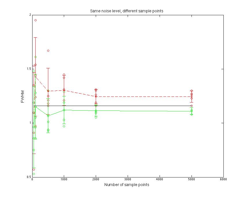
Figure 1.2 FWHM value compare
FWHM value goes to be stable when sample points goes to 2000.
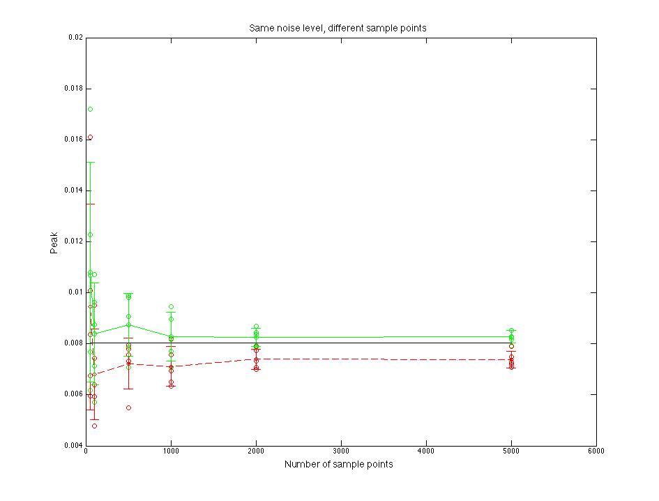
Figure 1.3 Peak value compare
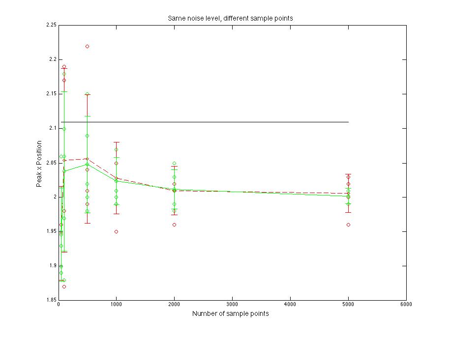
Figure 1.4 Peak x position value compare
2. Compare two
- For different sample points, 50,100,500,1000,2000,5000.
- Simulation loop 5 times(means sample 5 times, get 5 set of discrete data).
- Simulation model Lognormal, fitting model Lognormal.
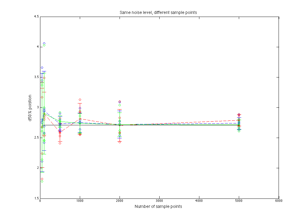
Figure 2.1 d50% value compare
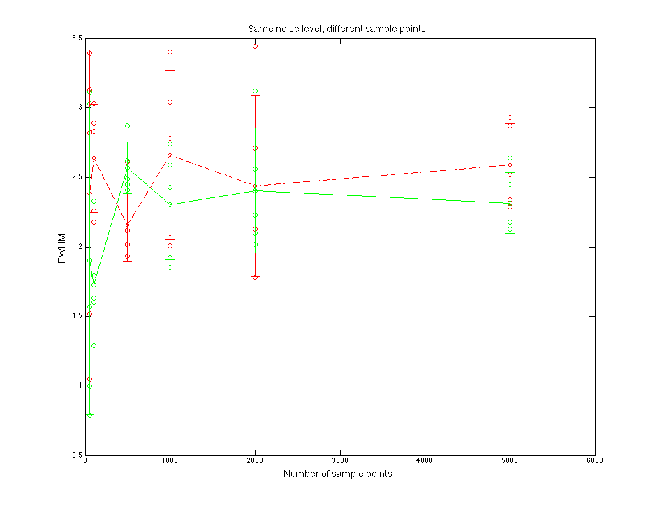
Figure 2.2 FWHM value compare
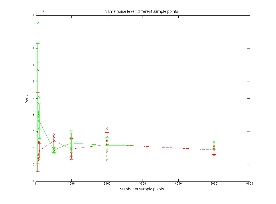
Figure 2.3 Peak value compare
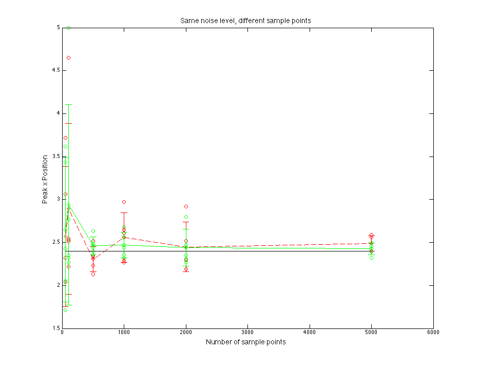
Figure 2.4 Peak x position value compare
3. Compare three
- For different sample points, 50,500,1000,5000.
- Simulation loop 10 times(means sample 10 times, get 10 set of discrete data).
- Simulation model Gaussian, fitting model Lognormal.
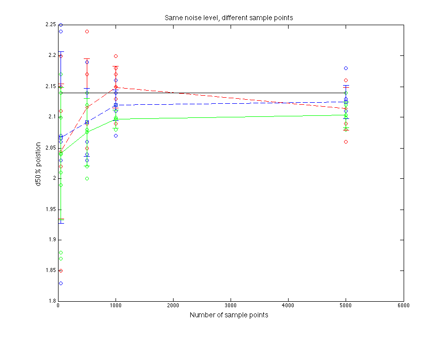
Figure 3.1 d50% value compare
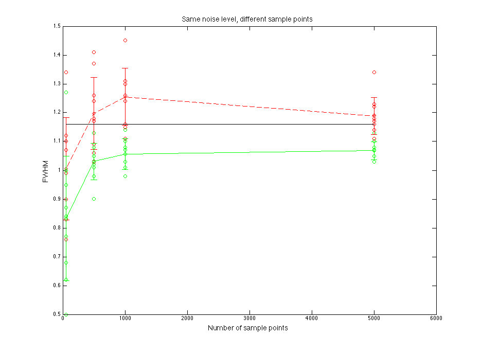
Figure 3.2 FWHM value compare
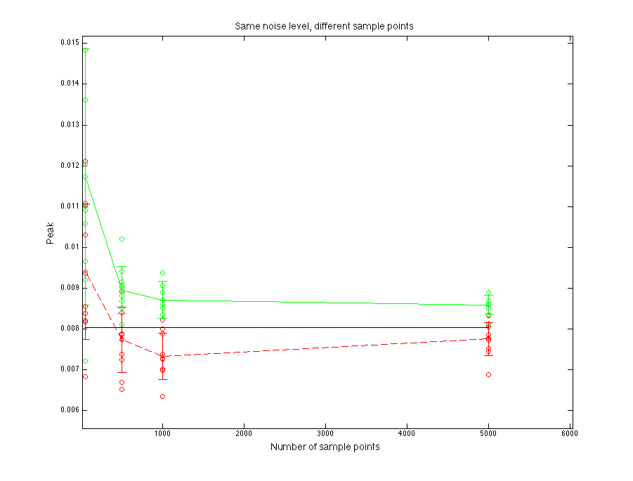
Figure 3.3 Peak value compare
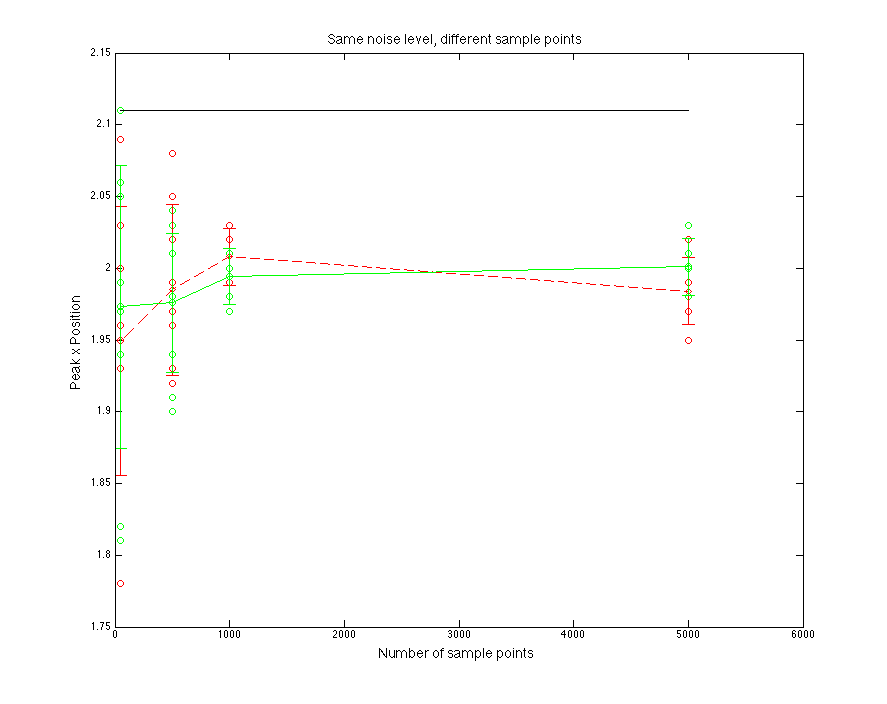
Figure 3.4 Peak x position value compare
4. Compare four
- For different sample points, 50,500,1000,5000.
- Simulation loop 10 times(means sample 10 times, get 10 set of discrete data).
- Simulation model Lognormal, fitting model Lognormal.
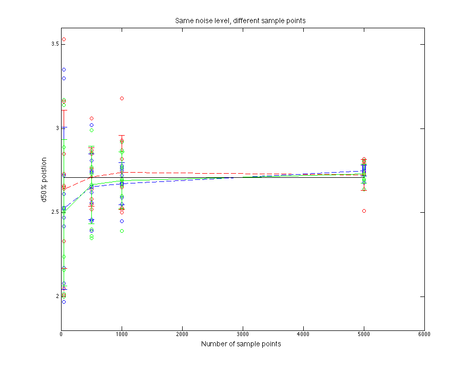
Figure 4.1 d50% value compare
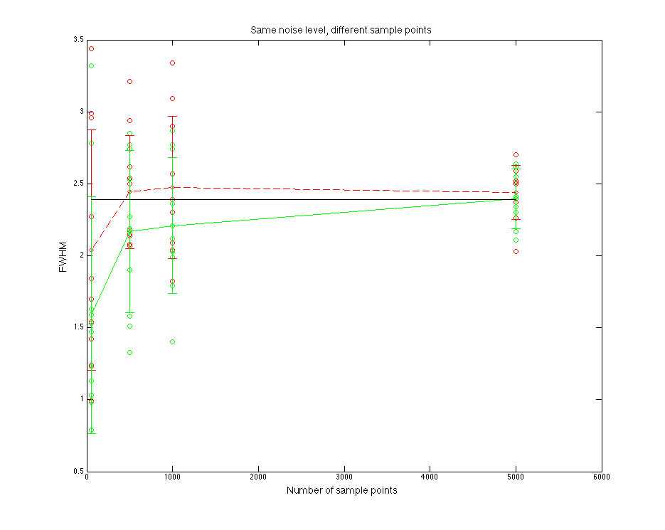
Figure 4.2 FWHM value compare
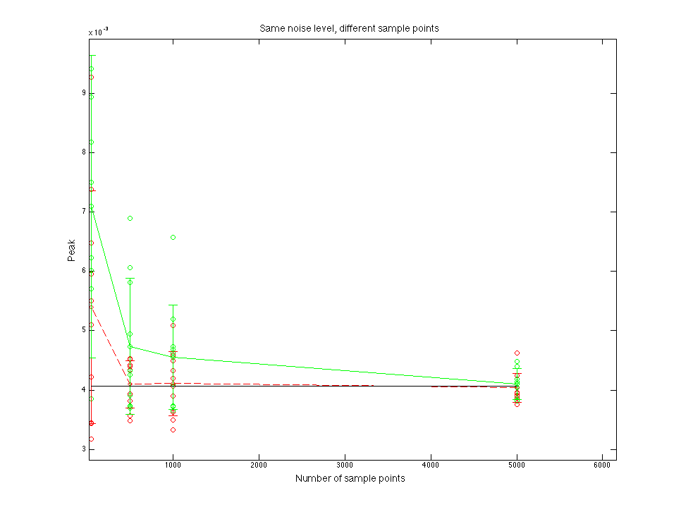
Figure 4.3 Peak value compare
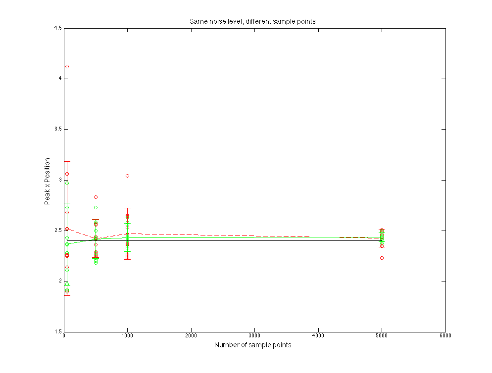
Figure 4.4 Peak x position value compare