DATA COMPONENTS
NVPT retrieves all the information from a .mat file called “Alldata.mat”, which contains information from the NIRS studies retrieved by the NIRS system Cephalogics LLC.
This “Alldata.mat” contains several elements related to the studies. The most important elements are:

Source(sources) .- A vector that has a series of purposely ordered and repeated numbers representing the all sources.
Detector(detectors) .- A vector that has a series of purposely ordered and repeated numbers representing all the detectors.
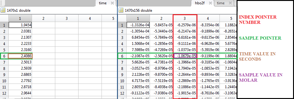
The position of the data inside the “Source” and “Detector” vectors is related to a unique source-detector separation, creating a reference pointer number (“Index” number) that is representing a possible nearest neighbor distance (NN1, NN2, NN3, NN4…) for the Oxihemoglobin, Deoxihemoglobin, 750 nm power signal, 850 nm power signal, etc., matrix’s.

Time(samples) .- A vector that contains the time value in seconds of every single sample.
hbo2f(samples,Index) .- A matrix that contains all the sampled values of oxihemoglobin concentration changes of all the possible nearest neighbor distances.
hbf(samples,Index) .- A matrix that contains all the sampled values of deoxihemoglobin concentration changes of all the possible nearest neighbor distances.
raw850data(samples,Index) .- A matrix that contains all the sampled and digitized values of 850 nm power signals of all the possible nearest neighbor distances.
raw750data(samples,Index) .- A matrix that contains all the sampled and digitized values of 750 nm power signals of all the possible nearest neighbor distances.
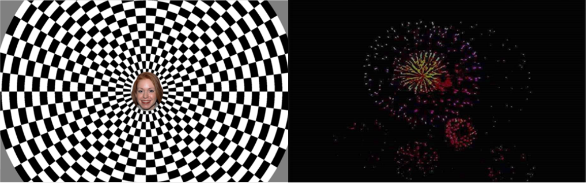
Start(start of stimulus sample) .- A vector that contains the pointer numbers of the starts of a reversing checkerboard stimulus.
Stop(stop of stimulus sample) .- A vector that contains the pointer numbers of the stops of the reversing checkerboard stimulus.
MATLAB FUNCTIONS
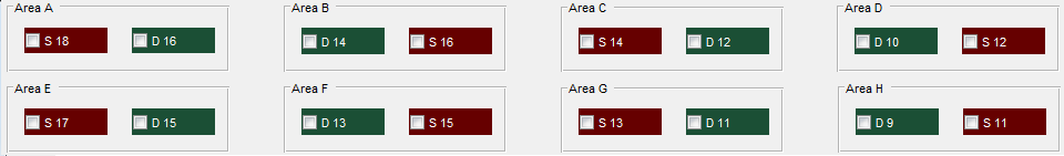
We proposed two matrices that imitate the sources and detectors positions in the probe, the distribution can be set with any desired geometry, this pair of matrices will be responsible for the logic of the source-detector selection for any future operation. in the probe F we have the next design that imitates the current geometry:
SourArr=[18 16 14 12;17 15 13 11];
DetArr=[16 14 12 10; 15 13 11 9];
We also need to create a Index Pointer Matrix that will contain the channel number for any possible source-detector distance. For this to happen, we use the positions of the numbers on the “Source” and “Detector” vectors to relate them in an easy way.
for(j=1:length(Source))
for(i=1:length(Detector))
SDindex(Source(i),Detector(i))=i;
end
end
SDindex(size(SDindex,1)+1,size(SDindex,2)+1)=0;
The last line of code is to give an “easy to use” zero value, It will be explained in the future. It’s necessary to understand that the intersection between a source and a detector on this matrix is a channel column number on the “hbo2f”, “hbf”,”raw850data” and “raw750data” matrices.

The logic that relates the selected Sources and Detectors in the NVPT User Interface, the “SDIndex” matrix and the “hbo2f”, “hbf”,”raw850data”, “raw750data” matrices are the “Boolean relationships”. This relationships defines what kind of nearest neighbor distance is happening or selected. The design of this logic was using strings and the function “strcat”.
First we design the logic for single distance taking as a unique reference the “SourArr” and ” DetArr” geometry. The sources and detectors in probe F geometry have 2 rows and 4 columns each. Forward on the code 4 nested cycles will be used with the variables “j”,”t”,”i”,”s” to obtain and calculate all the possible selected channels by the user. Using “j” and “t” for the columns, “i” and “s” for the rows. Remembering “SourArr” and ” DetArr” geometry :
SourArr=[18 16 14 12;17 15 13 11];
DetArr=[16 14 12 10; 15 13 11 9];
An NN1 channel in the current model supposes that the Source have the same location as the Detector, or an NN2 channel has the source or the detector to the left or to the right, therefore:
MM5 = ‘(j==t)&&(i==s)’;
MM20 = ‘((j==t+1)&&(i==s))||((j==t-1)&&(i==s))’;
MM21 = ‘((j==t)&&(i==s+1))||((j==t)&&(i==s-1))’;
MM28 = ‘((j==t+1)&&(i==s+1))||((j==t-1)&&(i==s-1))…
||((j==t+1)&&(i==s-1))||((j==t-1)&&(i==s+1))’;
Now that the basic nearest neighbor distances have been designed, is possible to design the “possible combinations”, in this case, there are 4 nearest neighbor distances, so there are 16 “possible combinations”.
DistStr{1}=strcat(MM28,’||’,MM21,’||’,MM20,’||’,MM5);
DistStr{2}=MM5;
DistStr{3}=strcat(MM20);
DistStr{4}=strcat(MM5,’||’,MM20);
DistStr{5}=MM21;
DistStr{6}=strcat(MM21,’||’,MM5);
DistStr{7}=strcat(MM21,’||’,MM20);
DistStr{8}=strcat(MM21,’||’,MM20,’||’,MM5);
DistStr{9}=MM28;
DistStr{10}=strcat(MM28,’||’,MM5);
DistStr{11}=strcat(MM28,’||’,MM20);
DistStr{12}=strcat(MM28,’||’,MM20,’||’,MM5);
DistStr{13}=strcat(MM28,’||’,MM21);
DistStr{14}=strcat(MM28,’||’,MM21,’||’,MM5);
DistStr{15}=strcat(MM28,’||’,MM21,’||’,MM20);
DistStr{16}=strcat(MM28,’||’,MM21,’||’,MM20,’||’,MM5);