For today’s group meeting, only the IRAM members (Xing, Robert, and Ashley) were in attendance. We primarily discussed the big picture scope of our project and the upcoming Photonics West presentations. Read More “Group Meeting 10/23/15”
Author: admin
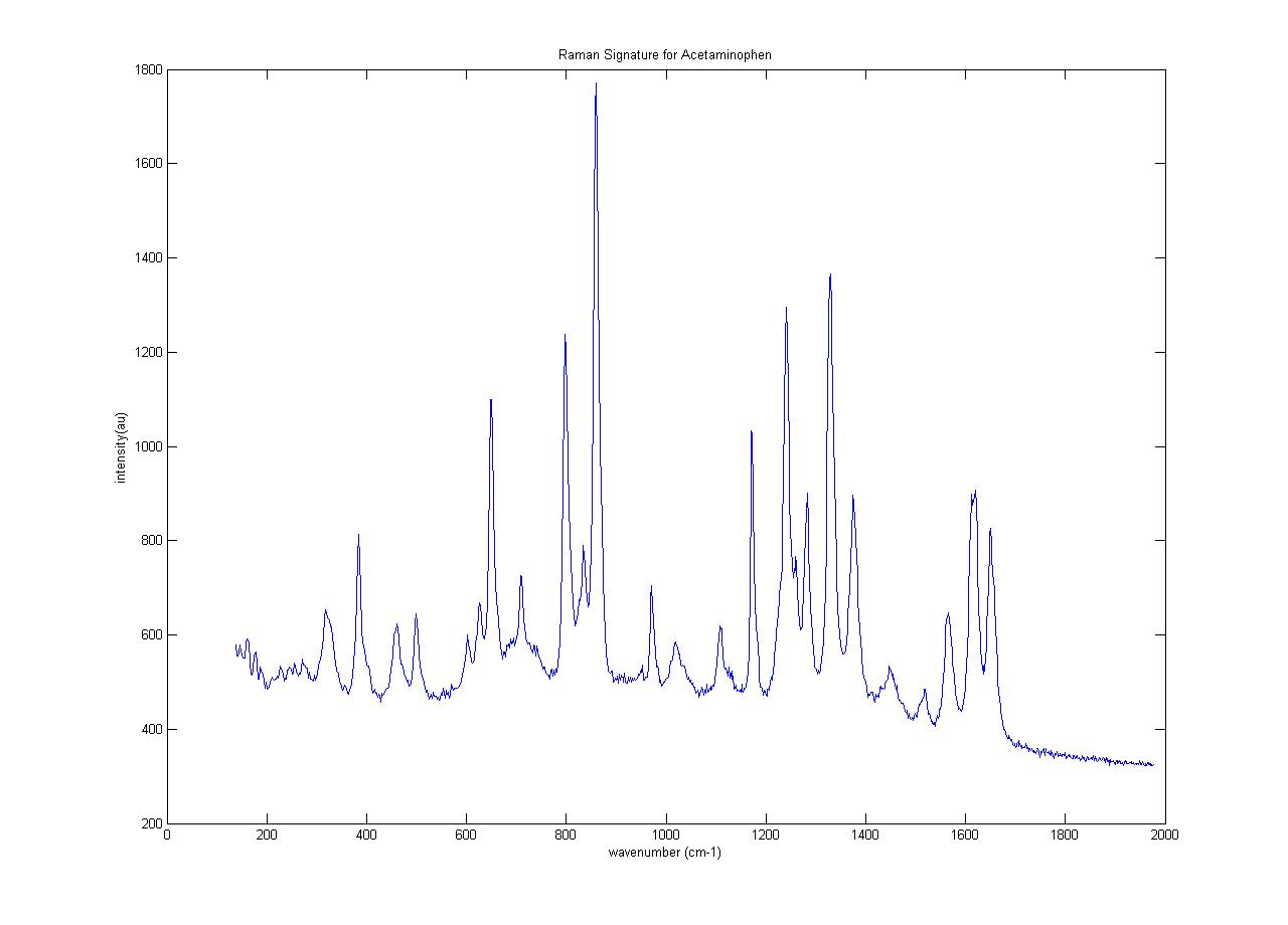
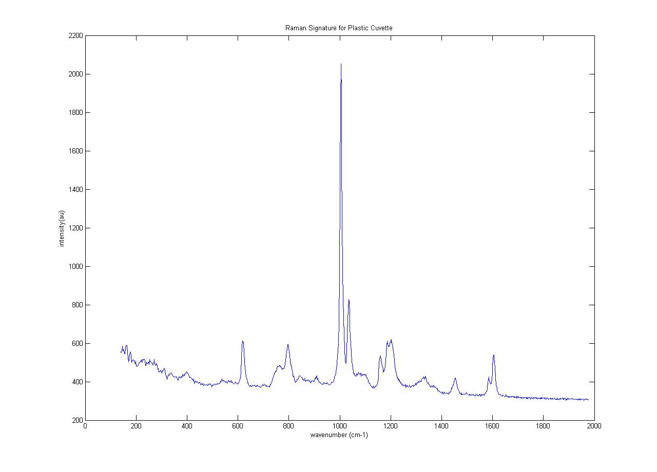
Raman Signature for Plastic cuvette and Acetaminophen using Confocal Raman Microspectroscopy system
Throughput vs angle correction
To our knowledge, the throughput of our system versus angles has not previously been accounted for. To determine it, we placed the teflon cap in the sample chamber, submerged it in water and put a square coverslip on top, just as we would for a bead sample. The scattergram for the cap is shown below.
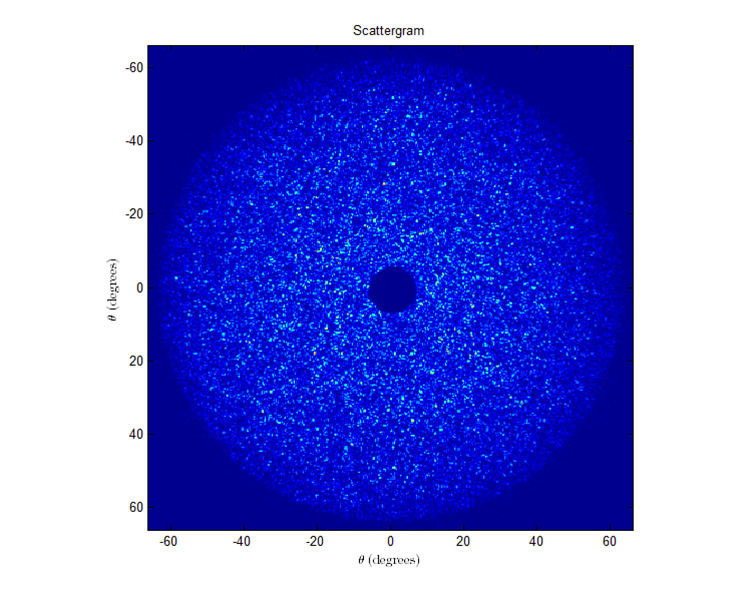 If the throughput did not change versus angle, then the intensity should be about constant (with noise) throughout the entire scattergram.
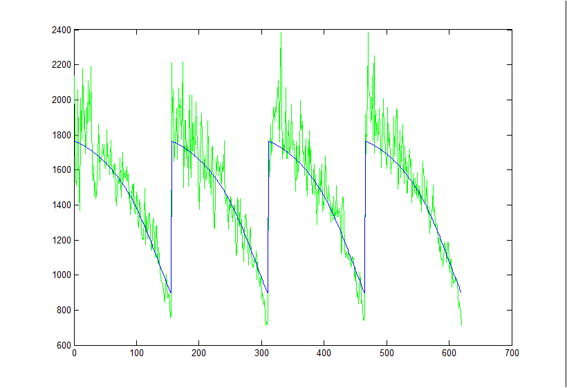
 However, we can tell from the cut-throughs that there is indeed a falloff. This falloff can be well fit to a cos(theta) function: Throughput(θ)=I(θmin)cos(θmin)cos(θ)
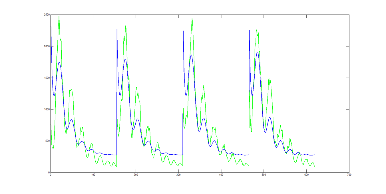
 Here is the least squares fit to a 5um bead without any throughput correction:
 And here is the fit with the throughput correction. The theory cut-throughs were multiplied by the above throughput equation and then least square fit to the data (with an offset and stretch term).
 The throughput correction did not have much of an impact on the quality of the fits. If instead you LSF the theory cuts to the data, like normal, and then multiply by cos(θ):
 The amplitudes of the peaks are still to small, but the falloff trend seems more correct.
Reference beam setup/alignment
- If pellicule beamsplitter is out, put it in between the CCD and the last lens of the 4f system. The engraved side should be facing away from the CCD. It should be at as much of a 45 degree angle as possible, given the space constraints. Make sure the beamsplitter is not clipping the sample beam.
- Direct the reference beam towards the CCD using reference mirrors 1 and 2.
- With all ND filters out, adjust reference mirror 1 so that the reference beam transmitted through the pellicule and the sample beam reflected off of it hit the same spot in the near field (close to the pellicule).
- Adjust reference mirror 2 so that the two spots overlap in the far field (farther away from the pellicule).
- When the spots are very close to overlapping, it may be beneficial to stop down both beams so that the spot sizes are small. Just make sure the iris’s used are centered!
- Put the ND filters back in, and make final adjustments to mirror 1 so that the two beams overlap perfectly.
- If this part of the alignment is correct, you should have circular fringes with good contrast.
- Put a sample of fixed beads into the system (larger beads make alignment easier).
- Place a bead on the edge of the elastic excitation beam, diagonal from the center. Adjust BS1 and reference mirror 1 so that the tilt fringes are nulled in the interferogram.
- Move the bead to the center of the excitation beam. Adjust the BS and mirror until the frequency of the tilt fringes approximately doubles in both x and y directions.
- Put in two pinholes along the reference beam path to make future alignments easier.
Wavelength and Raman shift calibration
Before data acquisition, the Wavelength and and Raman shift of the scattered light needs to be calibrated. A gas-discharged neon lamp needs to be used for wavelength calibration.
Wavelength Calibration:
Step 1: Taking spectrum data using neon lamp and then making plot of neon spectrum: Intensity vs. pixel.
Step 2: Using theoretical neon spectrum plot ( Intensity vs. wavelength) to identify neon peaks on the plot in Step 1 and making plot: wavelength vs. pixel.
Step 3: Making a third-order polynomial regression of the known wavelengths of neon on the corresponding pixel numbers.
Now, pixel numbers are able to be converted to wavelength by using the third-order polynomial relation.
Raman shift calibration:
Step 1: Taking spectrum data from any sample with known Raman shift spectrum(like Tylenol)
Step 2: Converting pixel to wavelength for Tylenol data and then plotting Tylenol spectrum: wavelength vs. pixel
Step 3: Using theoretical spectrum of Tylenol to identify peaks on the plot of Step 2 and save these peak points
Step 4: Using the equation: 1/laser wavelength = Raman shift +1/ wavelength of tylenol vibration to estimate the laser wavelength for each Tylenol vibration. Then take the average of laser wavelength.
Step 5: By using the equation in step 4 and the average laser wavelength, the wavelength is able to be converted into Raman shift
Short separation regression improves statistical significance and better localizes the hemodynamic response obtained by near-infrared spectroscopy for tasks with differing autonomic responses
Aligning the IRAM system
Raman alignment (all in epi-illumination mode):
1) With the air objective and no condenser lens, and a glass coverslip in the sample plane, use the 1st Raman mirror to make the two reflections from the coverslip overlap on the hitachi CCD.
2) With no objective or condenser lens, and a mirror facing downwards in the sample plane, use the 2nd Raman mirror to make the retro-reflection exiting the microscope hit the same spot as the illumination beam. (This can be done by using the IR viewer and a piece of lens paper to see both beams.)
3) Repeat steps 1-2 until they converge.
4) Put in the oil objective and a glass coverslip in the sample plane. Adjust the 2nd Raman mirror so that as the objective goes in and out of focus, the beam of the hitachi CCD has equal power in each quadrant of the spot.
5) Put in two pinholes after the periscope. These pinholes designate the path of a vertical beam.
Elastic alignment (in trans-illumination mode):
6) Use the two Elastic mirrors to direct the beam through the pinholes before the periscope, using the 1st mirror to align to the first pinhole and the 2nd mirror to align the second pinhole.
7) To fine-tune the beam so that it is going through the center of the objective with no condenser lens: Adjust the 2nd Elastic mirror so that the beam is hitting the center of the objective (will need IR viewer to see this). Then adjust the 1st Elastic mirror so that the beam is still going through the pinholes before the periscope. Repeat until the two converge.
8) Put in the condenser lens, and adjust its focus and position.
Quick Alignment
1) In epi-mode: Adjust 1st and 2nd Raman mirrors so that the beam is going through the 1st and 2nd pinholes, respectively, in the Raman excitation path.
2) In epi-mode: Without the condenser or objective, adjust the periscope mirrors so that the beam is going through the two pinholes after the periscope.
3) In trans-mode: Adjust the 1st and 2nd Elastic mirrors so that the beam is going through the two pinholes before the periscope.
4) Put in the objective and condenser. Adjust the focus and position of the condensor.
Compare normal fitting with direct fitting
These days work are mainly about comparing the performance of normal fitting and direct fitting.
A review for whole process. We have a parent Gauss or Normal distribution(parameter μ and σ). In math that should be continuous. Then we sample the distribution got a set of discrete data. Then we use the discrete population to map to a set of scattergram that generate by Mie scatter thoery in different particle diameter. After that we use cross-section to weight the data. Now we get the raw simulation data we use in normal fitting.
In normal fitting we use log-normal population model + cross-section weighted model+Mie theory to fit to the scattergram. We want to report best estimate of I vs d.
For direct fitting, the raw simulation data generate is similar to the former one. We have a parent Gauss or Normal distribution(parameter μ and σ), then we sample the distribution get a set of discrete data. We weighted these data though cross-weighting model. Now we get the raw simulation data.
In direct fitting, we use a log-normal or gaussian population model to fit raw data directly(without Mie thoery, that is why we call it direct fit).
The purpose of normal fitting is we want to analyze cell’s angular scattergram we taking from our experiment devices. We would like to report best estimate of I vs d.
The purpose of comparing these two fitting process is we want to know several things: how well our normal fit compared to the direct fit; when the samples are very sparse, the Mie thoery model’s contribution could be neglected, and so on.
Followings are several simulation results for comparing direct fitting and normal fitting. Read More “Compare normal fitting with direct fitting”
Cell culturing protocol
Thawing Frozen Cells
- Cells arrive deep-frozen.
- Add cells to 10 mL of growth media with 20% FBS.
- Incubate overnight or until confluent.
- Passage to 2 dishes with 10 mL of growth media with 10% FBS
- Continue to passage about twice a week.
Passaging (SCC7)
- Aspirate (remove) media.
- Add 1 mL of trypsin, coating the entire bottom of the dish.
- Swirl for 20 seconds, then aspirate.
- Add 1 mL trypsin.
- Incubate for 4 minutes.
- Use the pipette to “pressure wash” cells off of one dish with trypsin.
- Add the trypsin with the lifted cells to the second dish.
- Use pipette to wash cells off of the second dish with trypsin.
- Add (x) μL of trypsin with lifted cells to new dishes with 10 mL of growth media.
- (x) should be somewhere between 75 and 150, depending on how quickly you want the cells to reach confluence
Passaging (HeLa)
- Aspirate (remove) media.
- Add 10 mL of HBSS or PBS.
- Aspirate.
- Add 2-4 mL trypsin.
- Incubate for 3 minutes.
- Use the pipette to “pressure wash” cells off of one dish with trypsin.
- Add the trypsin with the lifted cells to the second dish.
- Use pipette to wash cells off of the second dish with trypsin.
- Add (x) μL of trypsin with lifted cells to new dishes with 10 mL of growth media.
- (x) should be somewhere between 75 and 150, depending on how quickly you want the cells to reach confluence
Cell Media/Solutions
Cell Media (EMT6)
- 500 mL BME (Basal Medium Eagle. We have always gotten this from the Foster lab)
- 2.5 mL Pen Strep
- 2 mL Fungizone
- 1 mL plasmocin
- 1 mL primocin
- 10% FBS – 55.5 mL (Fetal Bovine Serum)
*Note: 20% FBS media is also needed for when cells are first thawed.
*For SCC7 cell line, components are all the same except instead of BME base media, use RPMI media
Cell Media (HeLa)
- 500 mL RPMI 1640
- 10% FBS (50 mL)
- 5 mL Hepes Buffer
- 5 mL Pen Strep
*All Nada solutions are based on 500mL total final solution
Nada Solution #1 (basic cell measurement solution)
- 3.9447 g NaCl
- 0.2199 g KCl
- 0.9008 g D-glucose
- 6 mL Hepes
- 0.0832 g CaCl2
- 0.0571 g MgCl2
Nada Solution #2 (permeabilizing solution)
- 3.9447 g NaCl
- 0.2199 g KCl
- 0.9008 g D-glucose
- 6 mL Hepes
- 0.476 g MgCl2
- 20 μM Ionomycin
Nada Solution #3 (calcium shock solution)
- 3.9447g NaCl
- 0.2199g KCl
- 0.9008g D-glucose
- 6mL Hepes
- 0.0888g CaCl2
SUPERFASLIGAND (for 100 ng/10 uL concentration)
- 5 ug of SFL
- 500 uL of HeLa Media